
The Sprint: Automated Calibration of the SCREAM Model
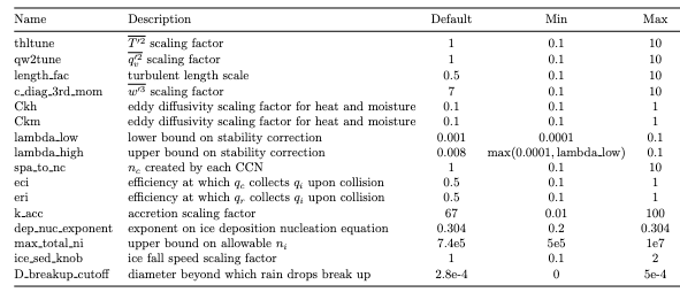
Figure 1: Calibration Parameters used in this study.
E3SM
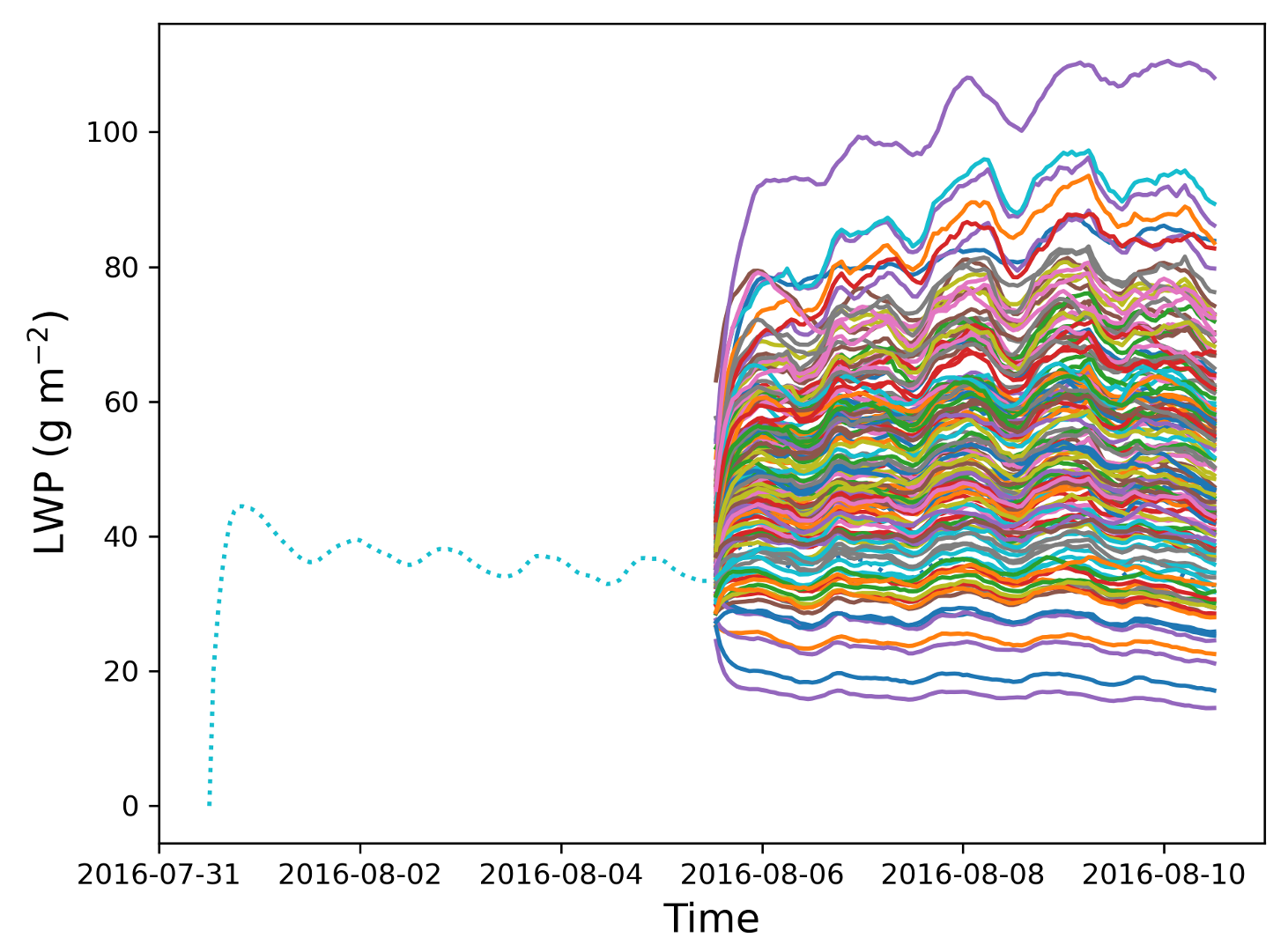
Figure 2: The team used a 5-day run nudged to ERA5 as the initial conditions for their 150-member perturbed parameter ensemble, before running foward for 5 more days. Here, global LWP is shown.
E3SM

Figure 3: Rendering of clouds from a SCREAM simulation.
Kuhn and Roeber (NVidia)
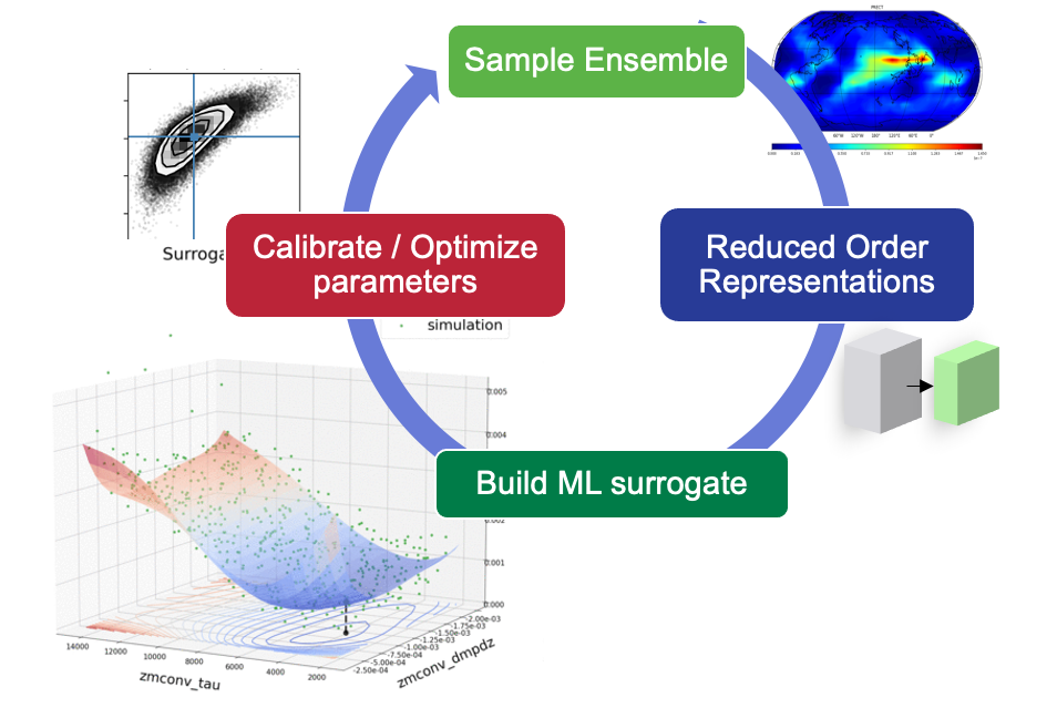
Figure 4: Workflow for automated calibration. While the generating of 150 samples was done once, the other three steps were done iteratively as the team refined the cost function.
E3SM
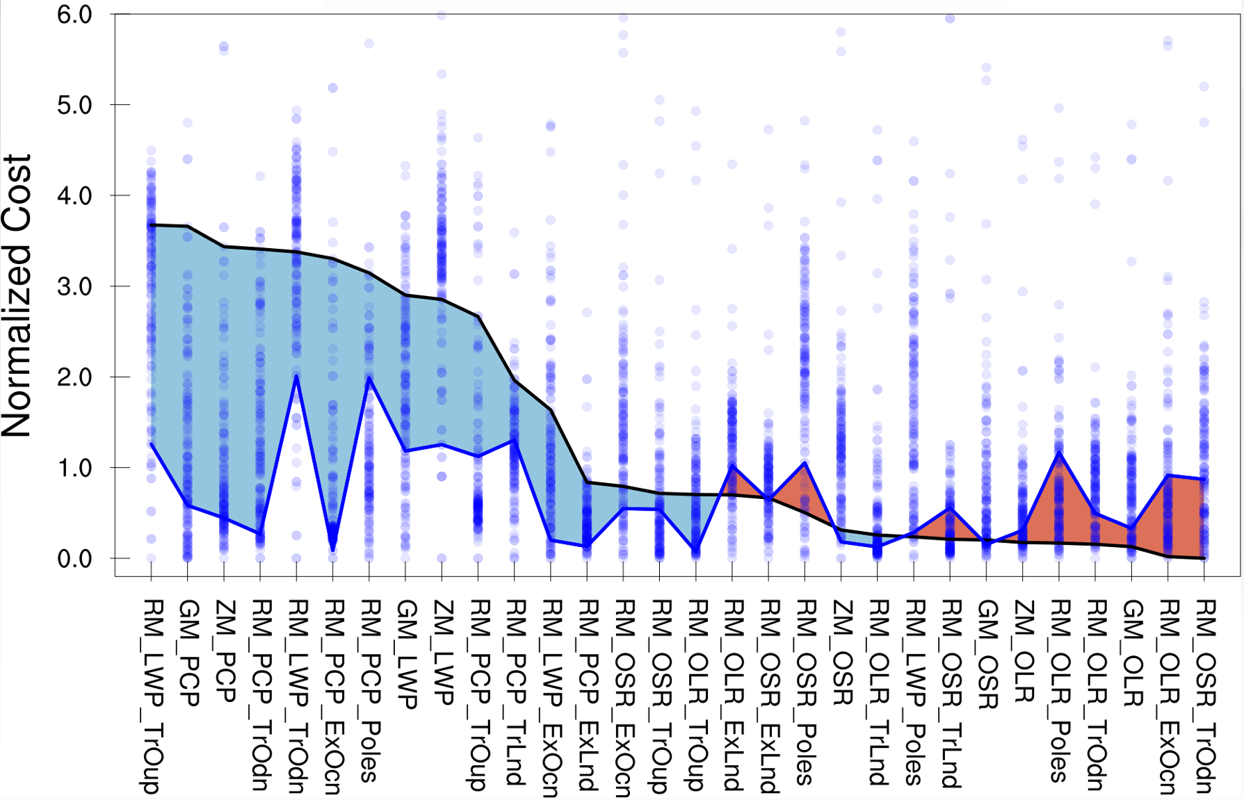
Figure 5: Model skill across a variety of metrics. Black Line=default and Blue line=optimized. Blue shaded areas indicate improvements in metrics with optimization, and red shows degradation.
E3SM
E3SM team members associated with the Exascale Computing Project (ECP) were presented with an opportunity this past December. To demonstrate the AI capabilities of the DOE Exascale systems, the ECP would extend the project and provide exascale computing resources if the team could produce novel scientific results using both exascale and machine learning (ML). The window for this opportunity was just three months.
The team proposed a project to perform automated calibration of the new SCREAM model.
- SCREAM clearly met the requirement for using exascale resources, with a documented ability to achieve over 1 simulated year per day on Frontier for a 3.25km (“cloud-resolving”) grid.
- The Automated Calibration effort within E3SM could meet the ML requirement, having used machine-learned surrogates as a key step in optimizing atmosphere physics parameters for E3SMv2 and v3.
- Was it possible to do something scientifically significant, and in three months?
In January, the 90-day sprint began. Peter Caldwell quickly took on the leadership role, establishing the key phases of the project, each with parallel efforts, with deadlines and deliverables. Typically 20-25 team members attend the weekly meetings, and it was not uncommon to have 100 Slack messages in a given day as the team rallied around the effort.
Scientific and Computational Hurdles
How to set up a calibration problem that was achievable within the time frame and computational resources? SCREAM requires a full exascale machine to run a simulated year in a day. Previous automated calibration runs for low-res E3SMv3 were built on several thousand years of simulation and climate metrics that were seasonal averages over multiple years.
The climate scientists on the team decided to focus on parameters that affect clouds, and use cloud properties as the climate calibration metrics, since they are known to emerge quickly in just a few days simulation time. Sixteen parameters – mostly from P3 (the Predicted Particle Properties microphysics parameterization) and SHOC (the Simplified High Order Closure turbulence closure parameterization) packages — were chosen as the tuning parameters. Four climate metrics (aka climate variables) were chosen from observational record that the team would attempt to fit: Outgoing Short Wave Radiation, Outgoing Long Wave Radiation, Total Liquid Path, and Precipitation. The simulation would use ERA5 observational data for the initial conditions and the observations.
How to execute the Perturbed Parameter Ensemble? The Automated Calibration team used Dakota Latin Hypercube sampling software and workflow to create large ensembles of runs at different parameter values, using the parameters and ranges in Figure 1. In the end, simulations were run at more than 150 different parameter sets, and for each parameter set, two simulations (starting in two different seasons) were run. Each SCREAM run simulated 2-5 days.
Figure 2 shows a spaghetti plot of an ensemble for Liquid Water Path (LWP) versus time showing the trajectories of 150 samples. The initial conditions at default parameter values were first run for 5 days, nudged to ERA5 observations, before the parameter values were then perturbed and the simulation ran 5 additional days. It is clear from the spread of the responses to the change in parameters that the parameters have significant impact on the LWP variable.
How to perform 300 individual runs in a few weeks? One hurdle that became instantly apparent was that SCREAM initialization time was slow: starting a run up to the point where it starts timestepping could take as much computational time as performing a few days of simulation. The EAMxx developers jumped on this and got the costs down to a manageable level.
The main obstacle was getting the jobs – a previously unattempted volume of runs — through the queues on Frontier. A typical request was for 6144 Frontier Nodes, bundling 12 ensemble members together, each using 512 Frontier Nodes (2048 GPUs). We were able to get excellent throughput, with our first 150 ensemble members computed in about a week of calendar time, due to the heroics of team member Noel Keen. The code and machine were both found to be very robust, with few failures.
How to choose a cost function to minimize? Even after choosing the four climate variables to minimize by choosing optimal values of the 16 tuning parameters, there were still many choices to make. For each variable (Outgoing Short Wave Radiation, Outgoing Long Wave Radiation, Liquid Water Path, and Precipitation), there were several options on how to define a metric. They could attempt to match 2D fields of these variables, 1D zonal averages, regional averages over 6 distinct regions of the earth surface, or global means; and for each there was the choice to attempt to match probability distributions (such as PDF of precipitation intensity) and not just means. In addition, each metric could be given a different weight, such as giving the tropics bigger weight than the poles; or different scale, such as taking the square or square-root of a metric to change how much a larger variance between simulation and observation would be penalized.
In Figure 3, the very detailed cloud patterns can be seen. When trying to match 2D fields as seen here, a slight horizontal offset of the appearance of clouds would correspond to a large error: a place with a cloud could be one grid point away from where a cloud is seen in observations, so both grid points would be penalized for poor skill. This led them to consider metrics with more averaging such as zonal means, and the efforts to choose a cost function became an iterative process with the next challenge they encountered: creating a surrogate and optimizing.
How to create a surrogate and identify optimal parameters? The Automated Calibration team had developed a workflow and software set for performing calibration, used previously on low-res (110km) models. This workflow is shown in Figure 4, with four main steps: ensemble generation, projection to a reduced basis, creation of a surrogate using ML algorithms such as polynomial chaos expansions, and finally optimizing the parameter values on the surrogate.
The challenge with SCREAM calibration was that calibrating root mean square error of 2D fields turned out not to be a well-characterized cost function, as detailed above. The team quickly adjusted the code base to be able to handle very different cost functions, weights, and scalings. Numerous iterations of defining cost functions, recalculating surrogates, and optimizing on the new surrogate, were performed over a few days. This is another area where heroic efforts over short windows of time allowed the sprint to succeed.
Final Result
In the end of this iteration of choosing a cost function and optimizing using ML, the team chose a cost function comprising of 30 metrics. Figure 5 shows the relative cost for those metrics, both for the default parameter and for the optimized parameters, where the metrics are sorted in descending order their cost at the default values of parameter. The blue region corresponds to improvements in climate metrics due to the calibration, while the red areas showed some metrics that got worse. Clearly the net cost is decreased (more blue area than red), corresponding to an improved calibration based on these metrics.
Take-Aways From the Sprint
- The team was able to improve the calibration of SCREAM in matching observations for cloud-related metrics.
- Everyone involved with the sprint found it very rewarding. Many team members went above-and-beyond to develop codes and tools on a rushed timeline.
- The team was only able to achieve these results in such a short time because of the robustness of the SCREAM code across a wide range of parameter values, the Frontier computer, and the automated calibration software.
- The team learned a lot about how to design simulation campaigns, and even codes, with automated calibration in mind.
- There is a mental shift from calibrating by “Choose parameters to give the best overall climate” to “Choose a cost function that, when minimized, will lead to parameters that give the best overall climate”. Both require expert judgement on the relative importance of matching different metrics, but the workflows are different.
- Sprints can be useful for high-productivity and tight focus for periodic need, but would not be sustainable for the long-term.
The scientific results of this sprint are being written up for publication in a journal article
The Team
Peter Caldwell (Lead), Andy Salinger (author of this article), Luca Bertagna, Hassan Beydoun, Gavin Collins, Peter Bogenschutz, Andrew Bradley, Aaron Donahue, Oksana Guba, Walter Hannah, Ben Hillman, Noel Keen, Jungmin Lee, Wuyin Lin, Hsi-Yen Ma, Naser Mahfouz, Lyndsay Shand, Mark Taylor, Chris Terai, and Benjamin Wagman.
We would like to acknowledge with appreciation: ECP/ASCR for funding the effort and supporting with computational resources; the patience of E3SM and other projects who lost the attention of many staff for three months; and the whole E3SM team and BER/ASCR sponsors for laying the foundation so that this work was possible.
Some opinions expressed are from the author and may not represent the entire team.
# # #
This article is a part of the E3SM “Floating Points” Newsletter. Read the full May 2024 edition.